The Kelly Criterion Explained

Basic Intuition

When you’re putting money in some effort to receive more money back, i.e. a bet, you’ll need to find out how much of your money you should wager. You wouldn’t bet all your money unless you are 100% sure that you will win a bet and you would not bet any of your money unless you’re 100% sure you will lose the bet. Intuitively, you would only bet some of your money — and what “some of your money” amounts to depends on how likely you think the winning outcome is.

If you think the winning outcome is more likely to occur, you’ll bet more of your money, and if you think a losing outcome is more likely, you’ll bet less of your money. Think of the lottery — you never bet all your money on one lottery ticket because the chance of winning is infinitesimal. Using this intuition of betting more or less depending on the likelihood of a profitable outcome, we can begin understanding the exact amount to bet.

The Math

The math behind the Kelly Criterion is based on simple probability and manipulation. What is important to understand is the compounding nature of bets it assumes. What that means is that each bet and its profits feed into the next bet. If you bet $100 and get $110 back, that $110 is used entirely in the next bet you place. This compounding principle is essentially the same one that compound interest uses.

With that being established, let’s introduce some variables:

p — the probability that you win the bet
q — the probability that you lose the bet, which is just 1-p
b — the payout from a successful bet, determined from the betting odds
- This is determined as follows: if the odds are “x-to-y”, then b = x/y
- For example, if the odds of a bet are “3-to-1”, then b = 3/1 = 3.0
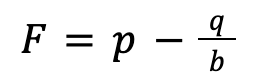
F — the optimal portion of your money you want to bet

Now that we have the variables, here’s the formula putting them together for a bet in which losing the bet means you lose the entire amount of money you bet:

Nothing shows how to use this formula better than a few examples. Let’s look at a few:

Example 1: Let’s say you flip a normal coin. Heads and tails both have a 0.5 (50%) chance of happening, so p = q = 0.5. If the payout of getting heads is “3-to-2” (if you bet $2, winning the bet returns you that $2 you bet plus $3 for winning the bet for a total profit of $5), then, b = 3/2 = 1.5. If you get tails, you lose what you bet.
- Plugging these into the formula, we get:

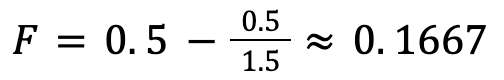
This means that given the payout from winning the bet (landing heads) and the probabilities of winning and losing the bet, you should only bet 0.1667, or ⅙, of your money. So if you had $100, you’d only bet $16.67 of it.

Example 2: Let’s say you win some money if you pull an Ace from a standard deck of cards. This has a 4/52 or 1/13 chance of happening, which means p = 1/13 and q = 12/13. If the payout of pulling an Ace is heads “12-to-1” (betting $1 and winning returns that $1 plus $5 for a total profit of $6), then, b = 5/1 = 5. If you get tails, you lose what you bet.
- Plugging these into the formula, we get:

This means that given the payout from winning the bet (getting heads) and the probabilities of winning and losing the bet, you shouldn’t bet anything because the payout from taking the risk isn’t worth it.

Incorporating Implied Probability

When making bets, it makes sense to factor in both the risk — the probability of losing your bet — and the reward — the payout from winning your bet. If one is less than the other, then it makes sense to at least bet some money because the odds are somewhat in your favor. With the lottery, if the odds are really small of winning, then to get people to actually play, the payout needs to be large enough to compensate for that enormous risk of not winning. When flipping a coin, the chance of flipping heads is the same as flipping tails, so to even flip the coin, you would want to make sure the payout is something that is net positive over many coin flips. Essentially, it all comes down to making sure the reward you may get adequately compensates you for the risk involved in the bet. How can we see this numerically?

It makes mathematical sense from the formula above that when p is greater than q/b, then it makes sense to bet some amount of money. If p is equal to q/b, then that means you’re likely to lose exactly what you make over many bets using the same payout and probabilities, so you shouldn’t bet anything. If p is less than q/b, then you’re likely to lose money over many bets, so you obviously shouldn’t bet any money.

Let’s dig deeper and understand why this makes more sense. To do so, we need to look at implied probability, which you can understand as the probability of an event occurring implied by the payout odds. In this case, the payout is b, so we can derive implied probability. If we have an “x-to-y” payout, the implied probability is y/(x+y). In other words, the implied probability is the amount you bet (y) divided by your total profit from the bet (x+y). So if you placed a bet with a “2-to-1” payout, then the implied probability of winning is 1/(2+1) = ⅓ = 33.3%. If you placed a bet with a “1-to-2” payout, then the implied probability of winning is 2/(1+2) = ⅔ = 66.6%. This makes intuitive sense since the greater the payout is, the more risky that bet is. It’s like the inversion of “greater risk, greater potential reward”. The idea is to find a payout with an implied probability that is less than the actual probability of winning. In Example 1, the implied probability of “3-to-2” odds is ⅖, or 40%. That is less than the actual probability of winning, which is just 50%. Therefore, it makes sense to bet some amount of money because the difference in implied probability and actual probability makes it profitable to do so.

Why is it profitable? Let’s again think about this intuitively by treating risk as a probability. If the payout’s implied probability is less than the actual probability, that means the payout is implying more risk is involved in that bet than actually exists. However, it is paying a reward based on the implied probability, which is greater due to a lower probability that implies that greater risk. Again, greater risk means greater potential reward. If a bet pays out a reward that implies a risk that is greater than the actual risk, then you’re more likely to get that reward because the probability of winning is actually higher. So for a lower amount of risk, you’re able to get the same reward as a higher level of risk. Taking advantage of this difference — this asymmetry in risk and reward — is what makes the bet worth making over the long-run.

So when the implied probability of winning is less than the actual probability of winning, it makes sense to bet some of your money. When the implied probability is greater than or equal to the actual probability of winning, it doesn’t make sense to bet any money. Following the same line of reasoning from earlier, if the implied probability of winning is greater than the actual probability of winning, it will pay a reward representing a more certain bet, which means that reward is smaller. As a result, the bet pays out a smaller reward for the actual level of risk involved. In other words, for a higher amount of risk, you’re getting the same reward as a lower level of risk. The reward doesn’t make the risk worth it. When both the implied and actual probabilities are the same, since the risk is equal to the reward, over many bets, the loss and growth — the risk and reward — essentially cancel each other out and leave you with the same amount of money as you started.

This idea of representing risk as a probability, finding a bet’s implied probability, and comparing it to the actual probability doesn’t stem from the Kelly Criterion. Rather, it’s what the Kelly Criterion, as well as many other betting tools, are based off of.

Maximizing the Growth Rate of a Bet

So we’ve introduced the formula for the Kelly Criterion, used it in a few examples, and tied it to the idea of implied probability. But, as previously stated, when the odds are in your favor, it definitely makes sense to bet some money. The Kelly Criterion tells you how much exactly to bet, but how? It boils down to the idea of maximizing the growth rate of a bet.

The formula given above for the Kelly Criterion did not start out that way and was arrived at through mathematical manipulation. It may look quite simple since it involves 3 variables and two elementary operations and no constants, exponents, logs, etc., but the actual way to derive it starts with a more complicated equation. Despite its seeming complexity, it actually makes a lot of sense if you remember that the Kelly Criterion is assuming compounding bets.

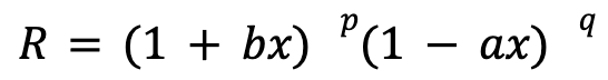
The idea of the Kelly Criterion is to find a proportion of your money that maximizes the growth rate of a bet. This means finding the optimal amount of money to bet so that you don’t bet too little and forego more reward and you don’t bet too much and lose more money when the losing outcome occurs. To find the growth rate of a compounding bet, we start by establishing the following using variables p, b, and q from earlier along with a new variable a:

The percentage your money grows when you bet x percent of your money and win
- When you win the bet, you get the payout of bx since b represents your payout per dollar bet
- Every time you win, your money grows by this amount. Since you have a p percent chance of winning, it makes sense to mathematically model the overall percentage growth from winning bets as follows: (1+bx)^p
The percentage your money falls when you bet x percent of your money and lose, which we’ll call a
- In bets where losing means losing the entire amount you bet, so a = 1, which corresponds to a 100% loss of the money that was bet
- Every time you win, your money falls by this amount. Since you have a q percent chance of losing, it makes sense to mathematically model the overall percentage growth from winning bets as follows: (1-ax)^q
R — the growth rate of a compounding bet

We can combine these different parts to find an equation that shows the relationship between the growth rate and the other variables. The equation is as follows:

What this essentially means is that the rate of growth you achieve over the long-run if you bet x percent of your money is directly proportional to b, a, p, and q. If b or p are large, you will achieve a higher rate of growth. If q or a are large, then your rate of growth will fall.

Using Desmos, I’ve created a graph that helps you see how R, or y on the graph, changes in relationship to the variables. You can check it out here: https://www.desmos.com/calculator/ndilewjmzr. On the x-axis, you have the fraction of your money — or bankroll — that you bet. On the y-axis, you have the growth rate that is achieved when a certain percent of your money is bet depending on the values of b, a, p, and q.

What you’ll see is that as you increase the values of b or p, holding the rest equal, you would end up betting a greater percentage of your money. Again, this makes sense because either the more reward you potentially make or the less risk you take, the more money you would bet. The opposite is true when q or a increases.

The x-axis is only limited to positive values because you can’t bet a negative percentage of your money. The y-axis, because the growth rates are represented by decimal values, shows values greater than 1 because values less than 1 imply your growth rate is actually negative. For example, if your growth rate is 0.9, that means over the long term, your bet changes by 0.9-1, which is -0.1, or -10%. This means your bet loses about 10% over the long-term. Feel free to play around with it!

Deriving the Kelly Criterion

From the equation above, we can derive the simpler relationship we found earlier. We want to find the percentage of money to bet to maximize the growth rate. This means we just have to find the derivative of the equation above and find where it equals 0. The derivation involves the following steps:

So, after applying a simple logarithm and deriving it, we get that the max growth rate is achieved when x = p/a – q/b, which is super simple! Again, when a = 1, which means that you lose the entire amount of money you bet if you lose, then we get the initial equation given: F = p – q/b.

Application to Investing

When making bets on outcomes where you lose all of what you bet, as described in the examples from earlier, the a variable is equal to 1. However, in investing, in which each investment can be viewed as a bet, it’s more often the case that you don’t lose all your money. The only way in which you lose all the money you invest is if, for example, the stock you invested in goes to zero because of bankruptcy. As a result, if you set a = 1, you’re expecting some unusually negative events to occur that wipe out the investment entirely. It’s more likely that an investment loses half its value, so if that’s what you expect, you could use a = 0.5 to represent the percentage of your investment you lose if the negative outcome occurs.

As you can probably begin to see, the Kelly Criterion can be incredibly useful in sizing the amount you want to invest. Let’s say you find an investment opportunity that you think will return 20% with a 60% chance and will lose 25% with a 40% chance. In this case, b = 0.2, p = 0.6, a = 0.25, and q = 0.4. Then, to maximize the growth rate of that investment, you plug those numbers into the Kelly Criterion formula as follows: x = 0.6/0.25 – 0.4/0.2 = 2.4-2 = 0.4. This means that in order to maximize your growth rate, you should invest 40% of your money in this specific investment.

If the investment instead has a 40% chance of dropping 10%, then a = 0.1, and the rest of the variables are the same. In that case, x = 0.6/0.1 – 0.4/0.2 = 6-2 = 4. In this case, you should bet 400% of your money, which implies you would have to borrow $3 for every $1 you bet of your own money. If leverage isn’t an option for you, then you would just invest 100% of your money in this investment. It makes sense to invest all your money because the investment essentially is delivering greater growth than loss with a greater probability of that growth.

Shortcomings of the Kelly Criterion

If the conclusion of investing all your money or investing with leverage from the example in the prior paragraph seems extreme, then you’d be right. The Kelly Criterion seeks to provide a definitive answer for your investment size, but that answer is based on you providing accurate values for the probabilities and magnitudes of growth and loss. So in order to use the Kelly Criterion to arrive at an amount to invest, you would need to possess incredibly accurate knowledge regarding future developments and confidently draw probabilities and magnitudes from that. It’s easy to know probabilities from a coin toss or from drawing cards, but it’s much harder to know the probability of, for example, a company’s new product growing to achieve market dominance or the probability of a distressed company refinancing its debt.

Overall, the Kelly Criterion tells you nothing about the accuracy and validity of the values used. The context in which you come up with those values determines that accuracy, and in the context of investing, finding completely accurate and precise values is, for all intents and purposes, pretty much impossible. Even if it was possible, the work required to find that out probably would cost so much time and money that using different risk management strategies is better. As Seth Klarman notes in Margin of Safety, the “value of in-depth fundamental analysis is subject to diminishing marginal returns”.

One solution to this is to estimate a range of values that could be used for the values in the Kelly Criterion and use the more conservative values in that range. Since any future event has a probability in between 0% and 100%, non-inclusive, of occurring, you could use a probability that represents a conservative bias rather than a probability that implies more confidence and optimism.

My personal opinion is to prioritize avoiding loss rather than chasing growth, so I’d take more conservative values for growth, which implies higher values for the loss variables. So if I think an investment has a 80% chance of returning 35% and a 30% chance of losing 50%, I would be conservative and use a number like 60% instead of 80% for the probability of growth and 25% instead of 35% for the magnitude of growth. This would lead to the Kelly Criterion telling me I should invest a lower percentage of my money in an investment.

Being conservative in your assumptions allows for a greater margin for error and ultimately protects you from sizable loss. Unless you’re absolutely certain you’ve done incredibly thorough research and analysis to come up with single numbers to represent the probabilities and magnitudes, I’d suggest using some conservative bias in your calculations using the Kelly Criterion.

Conclusion

The Kelly Criterion is an incredibly fascinating and useful method to use to arrive at the amount of money you should bet or invest. However, finding that amount to invest requires immense confidence in your ability to research and come up with precise and accurate probabilities and accompanying magnitudes. The Kelly Criterion’s seemingly fancy mathematics may give the illusion that its results are certain and absolute, but the inherent nature of investing means understanding the future is uncertain and that a formula is only as good as the values it takes. All that being said, the Kelly Criterion is still used by the most successful investors of our generation, and using it in your own investments may prove to be profitable. Good luck!